Quick Start Guide to 600A

Understanding the contractile function of muscle tissues (e.g., skeletal, cardiac, smooth) is imperative to many researchers within the muscle physiology and cardiology fields. As research advances, the scope of disease models of interest continues to broaden as well. Thus, there is a developing need to measure and quantify muscle contractility elicited by these tissues. The 600A Real-Time Muscle Data Acquisition and Analysis System is a powerful tool researchers can utilize to collect this muscle mechanics data.
The 600A software is a digital controller that allows researchers to precisely synchronize their equipment and record data in real-time. Unique features of this software include its ability to control force when using our high-speed length controller and force transducer in addition to measuring sarcomere length using our high-speed video sarcomere length system.
Table 1: Common research areas and products that employ the 600A Real Time Data Acquisition System
| Research Area | Research Model | Publications | Common Products/Systems |
|---|---|---|---|
| Muscle pathology & Wasting | Myopathy | Cardone et al., 2023 | 315D/322D, 400 Series, 1400A, 1500A |
| General Physiology | Cross-bridge kinetics, Thick & thin filaments | Tomalka et al., 2022 | 315D/322D, 400 Series, 901D, 1400A |
| Cardiology | Cardiomyopathy | Prondzynski et al., 2019 | 315D/322D, 400 Series, 950A, 1500A, 1600A, 1700A |
| Comparative Physiology | Single Fiber Mechanics | Wilson et al., 2018 | 315D/322D, 400 Series, 901D |
This technical blog will provide an overview on starting up the program, setup for tissues, loading and designing a protocol, opening the scope, starting a test, and analysis.
Jump to:
Start the Program
Here is a step-by-step guide to starting up the 600A software:
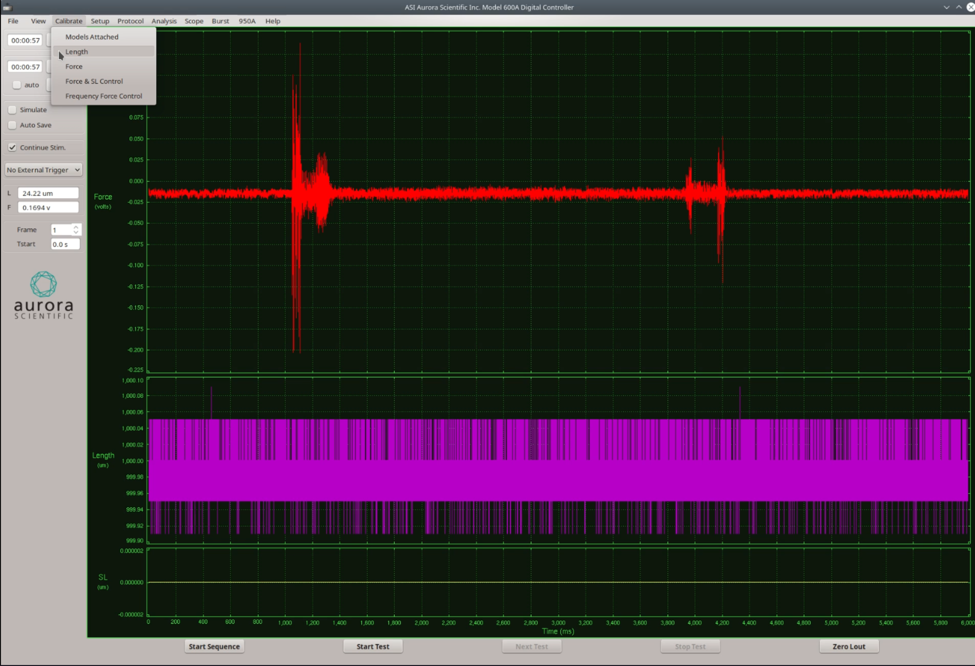
To start the 600A program, click on the icon labelled ASI600A. From the main window all menu items on the menu bar (File, View, Calibrate, Setup, Protocol, Analysis, Scope, Burst, 950A, and Help) are visible at the top of the screen. The bottom of the screen contains additional buttons to assist in running various tests. Key buttons to focus on are “Start Sequence” to starts a sequence of test protocols, “Start Test” to start a single protocol, “Next Test” to advance to the next test in a sequence, and “Stop Test” to stop a test protocol.
There are 6 text readouts located on the left side of the Main Screen. The first two timers can be used to time. The first two timers can be used to time experiments and to measure the time since the last stimulation. Below this, the input signals show the current values of Length In, denoted by the L and Force In, denoted by the F. These readouts are a convenient way to monitor the current state of the length controller and force transducer in addition to the Scope. The Frame number and Frame starting time (Tstart) in seconds are below this and can be used if the test protocol includes a Repeat function. The time indicates the start time of the Frame currently being displayed.
There are also Test buttons in the middle of this left side bar. The simulate button is used to check the timing of a protocol. If the simulate button is pressed, then when Start Test or Start Sequence are also pressed the output control signals and the Stimulus and Triggers will be displayed in the Main windows graphics area. No control signals will be issued to any of the instruments.
I will also draw your attention to the autosave button on the left side. When autosave is selected, data will automatically be saved to an autosave folder on the computer, after a test is completed. However, it is important to note that data is automatically saved when running sequences ONLY.
If you would prefer to manually save data following each test, this can be done after the test finishes by using the “File” ⇒ “Save Data” function.
Calibration

To maintain consistency between measurements collected via our hardware and software, it is important to calibrate your equipment following its unboxing and routinely afterwards. Calibration is imperative for maintaining accuracy, standardization, and repeatability between and within instrument measurements. If no calibration is done, it is likely the equipment can fall out of specifications, provide inaccurate measurements, and threaten quality of the equipment.
The calibration menu contains commands to set the selected lever system model and force transducer that will be used with the 600A software, to calibrate your length controller and force transducer, and to provide force and sarcomere length feedback control.
Please refer to our previous blog on how to calibrate your instruments using 600A.
Setup
To open the Setup window, Click on the “Setup” Menu heading and then click “Open”.
This window is divided into 5 sections ⇒ Set Reference Length, Fiber Cross Section, Other Parameters, Set Zero Load, and Notes.
Before entering any values into the Set Up window text boxes, the desired muscle tissue such as a single muscle fiber should be mounted.
Set Reference Length
The “Reference Length” refers to the length of the tissue that is mounted. For example, the fiber that is tied onto the pins of the length controller and force transducer. In this section, enter the muscle tissue length in the Reference Length text box and press the “Zero Lout” button. This will set the current position of the tissue as the ‘zero’ position and the program will use it as a reference to move back to. Now press the “Record Lin” button. The program will sample the current Length In value and display this value in mV, in the Lin (Length In) text box and in the Lref (Ref. Length) text box.
Please note:
- Fiber length units = mm.
- If the length controller or the stage position are changed at any time following the saving and closure of this setup window the reference length must be set again!
- Do not set Lo to zero!
- The initial length of your tissue is used in length control functions and if set incorrectly, the hardware will move unexpectedly. Lo should always be set to a positive, non-zero value.
Fiber Cross Section
Choose the type of cross section that is appropriate for your tissue, such as circular, rectangular or elliptical. Then enter the dimensions corresponding to the type of cross section you selected. The program will automatically calculate the Effective Diameter (Do) to give you the cross-sectional area (CSA) of a fiber for example.
Scope
Scope is a useful window that allows you to visualize the force and length data from your tissues in real-time.
Before running a protocol, you may want to open your scope. This window acts as a live-data monitor, resembling an oscilloscope. Scope can be open during all tests to provide long-term information about what length, force, sarcomere length, and auxiliary data has done over a period of up to 4 hours.
To open this tool, click on “Open” in the “Scope” menu.
Protocol
To open the protocol editor, select “Protocol” and then “Open“. In this window you can create various protocols, which control each function based on time. This pop out window can remain open during testing, which makes it easier to load individual protocols and observe their steps.
The four main headings associated with creating a protocol are: Step, Time, Function, and Parameters. Each protocol must contain at least 3 steps (data-enable, data-disable, and stop), but many more are able to be added depending on your research needs. All test protocols are created in order of steps, and each step has a start time, a function, and function parameters. A step cannot start before a previous step has completed. The program checks the protocol to ensure that each step starts at a later time, but you should still check to ensure that the function called on completes before the start time of the next step. The minimum time between instructions is set in the program to be 0.1 ms. So, when creating an instruction, it must have a start time that is a minimum of 0.1 ms after the time when the previous command finished. All functions start at the start time set, except for Stimulus and Trigger functions which are special and can have a delayed start.
Important things to note…
Each protocol must contain at least 3 steps, but many more are able to be added.
As each step is entered ⇒ the step number is automatically populated for you.
Ensure that Time increases for each successive step ⇒ the program has a built-in scan for this and will indicate if there is an error.
The help text at the bottom of the screen is a great resource when trying to understand each function (via brief description), its timing, and the parameters each function requires. As each step is clicked on, the box will update with its associated information.
When writing or inserting a protocol, important buttons include…
Insert ⇒ Inserts a line in the protocol at the highlighted location. The inserted line contains the same functions and parameters as in the highlighted line.
Append ⇒ Appends a line to the end of the protocol.
Up ⇒ Moves the highlighted protocol function up one position.
Down ⇒ Moves the selected protocol function down one position.
Delete ⇒ Deletes the highlighted line in the protocol.
Start Test ⇒ Starts the currently loaded protocol. This is the same button as the Start Test button on the main screen.
Load ⇒ Loads a protocol file saved on the computer. Once a protocol has been loaded, it can be executed.
Save As ⇒ Save As saves a protocol to a new file name. Any edited protocol file must be saved using either Save As or Save before the protocol can be executed
Save ⇒ Saves a protocol file to the currently defined protocol file name.
Protocol Functions
Controls
| Function | Description | Parameters | Example | Application in Research |
|---|---|---|---|---|
| Data-Enable | Start data collection | None | 0.0 Data-Enable | Required in all protocols written in 600A software |
| Data-Disable | Stop data collection | None | 100.0 Data-Disable | |
| Stop | Ends the test protocol | None | 350.0 Stop |
Length
| Function | Description | Parameters | Example | Application in Research |
|---|---|---|---|---|
| Step | Perform a step change in length | Absolute: [um, mm, Lo, Lf, volts] OR Relative: Prefix [- or +] | Absolute: 20.0 Length-Step 105.0 um (1.05 Lo) (step change the length to 105um) Relative: 20.0 Length-Step +5.00um (stretch by 5.0 um) | kTR (rate of force redevelopment) |
| Ramp | Perform a ramp change in length | Absolute: [um, mm, Lo, Lf, volts] OR Relative: prefix [– or +] AND ramp time [ms, s] | Absolute: 20.0 Length-Ramp 105.0 um 22.0 ms (ramp change the length to 105um over 22ms) Relative: 20.0 Length-Ramp -5.00 um 22.0 ms (shorten by 5.0 um over 22ms) | Vo (unloaded shortening velocity) OR Vmax |
| Sine | Change length using a sine wave pattern | Frequency [Hz], amplitude [um, mm, Lo, Lf, volts], duration [ms, s] | 20.0 Length-Sine 55 Hz 0.2 mm 0.12 s | Stiffness test |
Force
| Function | Description | Parameters | Example | Application in Research |
|---|---|---|---|---|
| Step | Perform a step change in force | Absolute desired force: [mN, N, gm, kg, Fmax, Pa, kPa, volts] OR Relative: prefix [– or +] |
Absolute: 20.0 Force-Step 25.0 mN (step change force to 25mN) Relative: 20.0 Force-Step +25.00 mN (Increased force by 25mn) |
RFE protocols |
| Clamp | Monitor force and when it reaches a specified value then clamp the force for a specified period | Clamp force [mN, N, gm, kg, Fmax, Pa, kPa, volts], delay time [ms, s], duration [ms, s] | 20.0 Force-Clamp 28.0 mN 50 ms 1.0 s (wait 50 ms then monitor force and when it reaches 28 mN hold the force for 1 s) | Load clamp (e.g., for cardiac tissue) |
Stimulation
| Function | Description | Parameters | Example | Application in Research |
|---|---|---|---|---|
| Stimulus | Start eliciting stimulus pulses (can modify which stim will be called in from the Stimulation tab) | Stimulation pattern number [valid range: 1-10], delay time [ms, s] | 20.0 Stimulus 1 5 ms (Note: stimulation profile is defined in Protocol ⇒ Stimulus) |
Stimulate tissue (e.g., pace cardiac tissue) |
Starting a Test
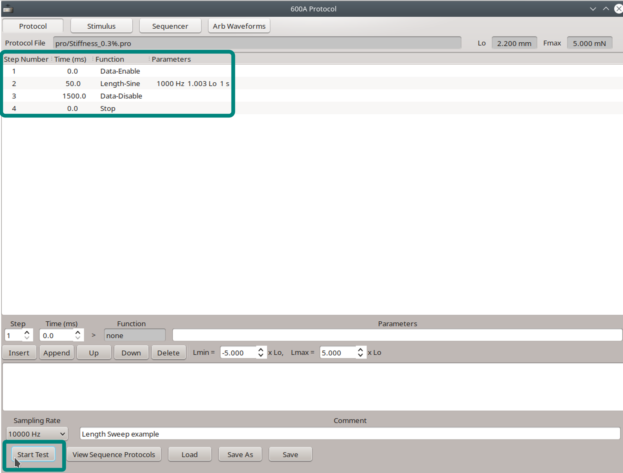
Before starting a test, you will need to open the protocol window. Please refer to the above section. Click “Load” at the bottom of this window to choose from the protocols that have been pre-loaded on the computer.
As an example, let’s load the stiffness.pro protocol.

For this protocol, the data will start collecting at 0ms, indicated by Data-Enable, a change in length of the fiber using a sine wave pattern (called a Length-Sine protocol) occurs at 50ms. In this protocol we are stretching the fiber 0.3% of its optimal length for 1s. The parameters of this particular protocol are as follows:
- Frequency = 1000 Hz
- Amplitude = 1.003 Lo (in terms of absolute control)
- Duration = 1 s
Then to stop collection, there is a Disable-Data function at 1500ms, followed by a Stop function at 1500.1ms.
Notice that there are steps, a time where each step starts, the function that will be done at that time, and the parameters which are provided in the text entry boxes.
Following the loading of a protocol, press the “Start Test” button at the bottom of the screen on either the main window or the protocol window.
The results of the test will show up on the main screen as soon as the protocol is finished. The graph that is visible is how the data is recorded and will be saved. If the protocol includes a “Repeat” function, then the results for each execution will be plotted immediately. If there is more than one pair of “Data-Enable” or “Data-Disable” functions, then each Data-Enable function will generate a new Frame.
Once the protocol is done, it can be saved to the desired folder by pressing “File” ⇒ “Save Data“.
Analysis

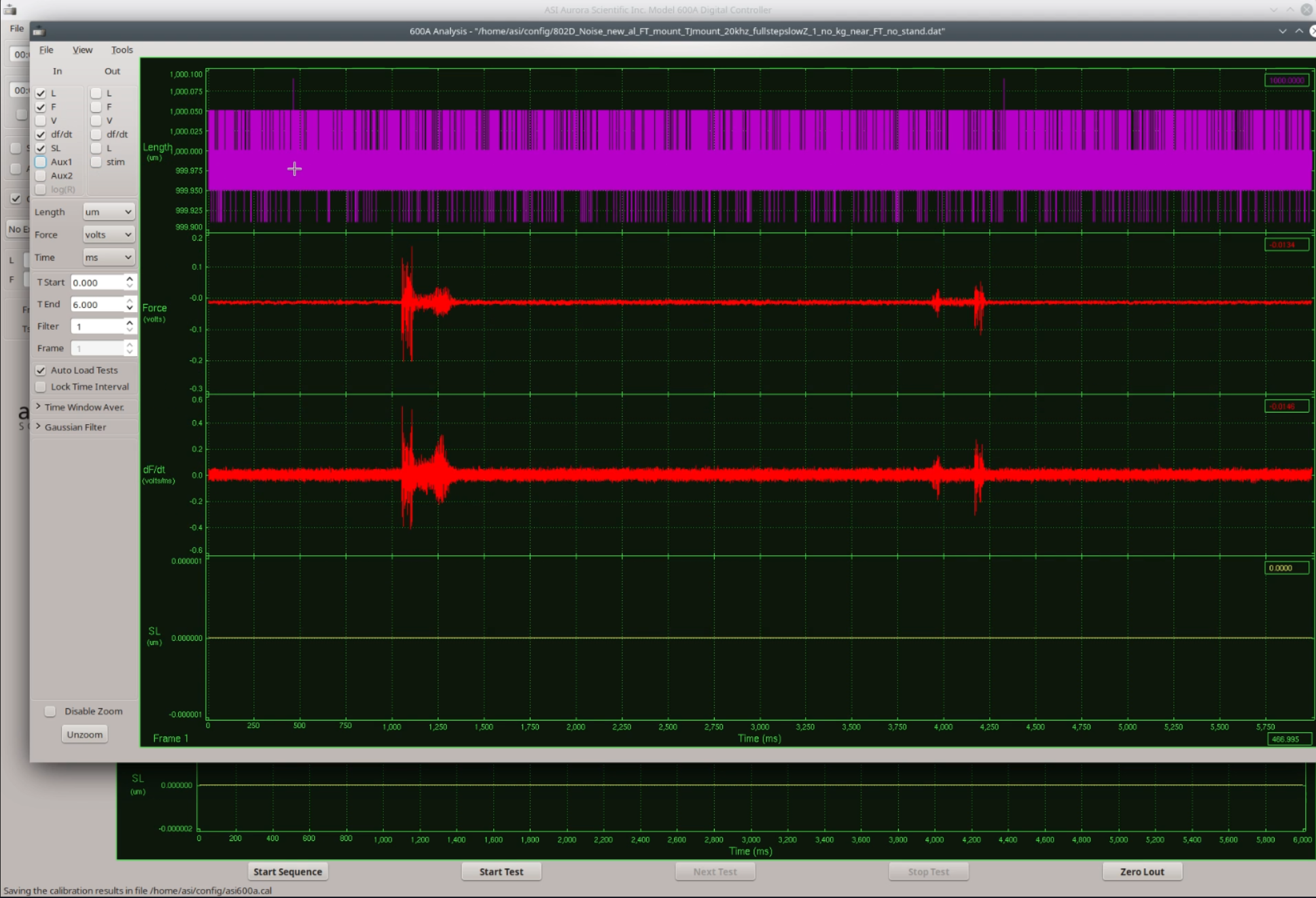
The analysis window can be used to review collected data stored on your Linux computer, zoom in on selected areas and perform calculations.
To open the analysis window, click on “Analysis“, then “Open“. From this window you an lead the most recent data collected or data that is saved on the computer.
Select the desired file (.txt) and click “Open“. This display will exhibit Length, Force, Velocity, dF/dt, SL, Aux1, Aux2 depending on the protocol and data collected during that time. Hovering your cursor over the force or length graphs will provide information with respect to the x and y axis (e.g., force at a specific length, following maximal activation).
To further analyze data collected in the 600A software…
- Files are saved as .txt
- These can be exported to your programming software of choice (e.g., MATLAB or python, to further manipulate the data)
Further Reading
Check out our blog on Tips and Tricks for using the 1400A Permeabilized Fiber System to assist you in improving the quality of your measurements and increase experimental throughput.
You can also check out our blog on Parameters to Setup in ASI600A Digital Controller Before Starting an Experiment, which is a step-by-step guide to setting up your high-speed length controller before commencing an experiment.
