Our High Throughput module of Dynamic Muscle Analysis has been a key part of Aurora Scientific’s systems for whole muscle and whole animal contractility for nearly 10 years. Over this time we have revised the capabilities and features of the program, so it is useful to revisit some of the nuances of the program from time to time to ensure you’re getting the most use out of the software. The following are a few of the most common and simple examples of ways to expedite analysis so you can get the most out of your contractility data.
Use Manual Cursors to analyze the active portion of an eccentric contraction
Eccentric contractions are commonly used as a means of inducing sarcolemma damage to help evaluate an intervention or animal model’s innate ability to maintain contractile strength under these conditions.
Briefly, an eccentric contraction begins by stimulating the muscle while holding it at a fixed length (isometric). Typically, the force will be allowed to plateau before inducing the stretch of the muscle. We could call this the active portion of contraction (see Figure 1). Once this plateau is achieved and the stretch of the muscle begins, we can observe a 2nd increase in tension which peaks at the apex of the stretch and will typically coincide with the end of stimulation. We would refer to this second phase of the contraction as the passive portion.
With each subsequent eccentric contraction, we would expect that the active force or the plateau region would decrease due to the sarcolemma damage accrued. We would not expect to see the same sort of change to the passive portion of the contraction as it solely represents the passive elastic properties of the muscle tissue. Thus, to truly quantify the effect of these contractions, we should assess the drop in the active portion of the contraction and not the absolute peak which includes the passive portion.
This poses a potential pitfall if we simply stick with the default settings of DMA and let the software automatically set the start and end cursors. The algorithm will always attempt to create a bound around the peak of the contraction (i.e. passive portion) and misrepresent the actual force deficit created from the eccentric contractions. To only measure the deficit of the active portion we should select manual cursors instead. The start cursor can then be set at time zero (to capture some baseline data) and the end cursor at the moment the stretch begins (in the case of Figure 1, 0.7s). It is quite typical to run a series of eccentric contractions, therefore we can analyze many traces at the same time using the batch analysis power of the high throughput module. To do this manually or a single file at a time would be a much more time-consuming affair.
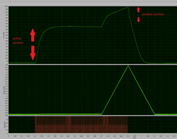
Figure 1: Typical Eccentric contraction showing each portion of the contraction.
Setting the correct reference for measuring ½ relaxation times in both twitch and tetanii
Isometric twitch and tetanii are the most basic and foundational measurements of contractile strength and thus are part of virtually every contractile experiment (with skeletal muscle). Performing measurements of ½ relaxation time (½ RT) is quite common and useful. It can tell us something about calcium kinetics, fiber type of the muscle and effectiveness of treatments for relaxation disorders (ie myotonia), among others. However, quantifying relaxation times requires a confident understanding of when the contraction truly ends and relaxation begins.
Compare the two images below. In Figure 2 we see a typical twitch contraction. A single stimulation pulse is generated, and then after a short delay contractile force begins to develop. The contraction peaks and then begins a rapid relaxation phase. It seems obvious that we should take the start of relaxation as beginning at this apex, which in fact we do for a single twitch. However, this is not always the case.
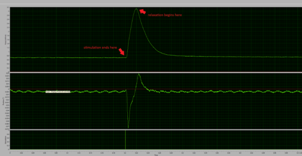
Figure 2: Typical Twitch Contraction.
In Figure 3 we can see a typical tetanic contraction. In some cases, contractile force may potentiate through the duration of stimuli with the peak occurring at the end of this stimulation train. However, the majority of the time (as is shown here) this does not occur. If we were to reference the start of relaxation as being from the peak force, we would erroneously and incorrectly measure the half relaxation time. In the case of all tetanii, we should reference the start of relaxation as being from the end of stimulation. Regardless of whether it is correct to reference relaxation as beginning from the peak of force or the end of stimulation, this can be changed in the analysis column settings as shown in Figure 4.
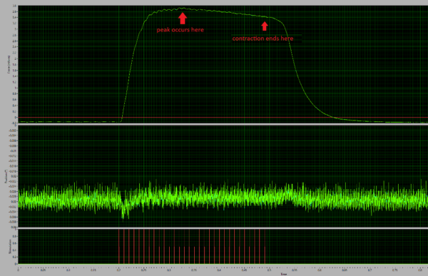
Figure 3: Typical Tetanus Contraction.
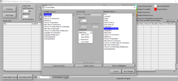
Figure 4: Edit Columns window showing ½ RT parameters.
Quantifying rates of contraction and relaxation
In the DMA High Throughput module there are default analyses which will calculate the maximum rate of contraction and relaxation. Essentially, these two columns will show the point on the contractile curve at which a tangent would have the highest absolute value (i.e. slope). While these values could potentially show broad trends in how rates of contraction or relaxation may compare between two cohorts it is not necessarily the best way to accomplish this. It is important to remember that this form of analysis represents one instantaneous data point on the entire curve. This point may not occur at the same time on all the traces that are under analysis. As a single data point, the outcome of the analysis is therefore very susceptible to noise or artifact and can even vary based on the sampling rate of the software!
A far better way to look at rates of contraction and relaxation would be to use the average rates of contraction/relaxation columns which can be edited and modified through the column editor window shown in Figure 5. Essentially, the average rate of contraction/relaxation function acts as a line fit between a user defined percentage of the maximum force (say 20% and 80%). The slope of the fitted line is therefore the average rate of contraction or relaxation.
This is a much better means of looking for changes in contraction or relaxation rates as it looks at a virtually identical slice of each contraction analyzed and works with a much larger data set. Additionally, thanks to the flexibility of the analysis parameters, you could even subdivide portions of the contracting or relaxing phase for a more detailed look.
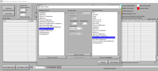
Figure 5: Edit columns window – showing average rate of contraction function.